A Literature Review of Speaker Change Detection

Introduction

Speaker diarization is the task of determining who spoke when in an audio stream, usually without knowing the number of speakers in advance. Speaker change detection is an important part of this problem. It aims to find the boundaries between the speech turns of different speakers.

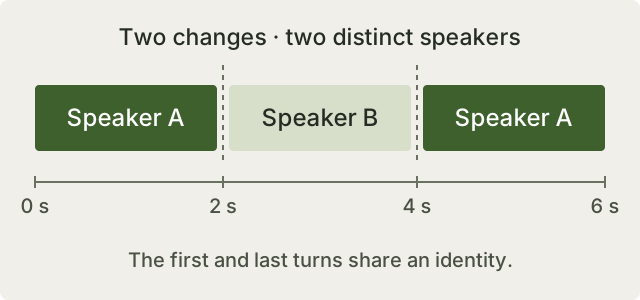
For instance, we may hear Speaker A, then Speaker B, and then Speaker A again. Finding the two changes is one task. Understanding that the first and last turns belong to the same speaker is another. Also, these labels do not have to tell us the person’s real identity.

In this post, I want to collect the papers I am reading and explain their main ideas. Some are directly about speaker change detection; others are about speaker embeddings, verification, or clustering. I include them because they can give us useful ideas for solving the diarization problem.

I will not cover every mathematical detail. My aim is to make the methods easier to follow, and I highly recommend checking the papers for their full explanations and results. If you would like to suggest another paper, feel free to get in touch. :)

Useful datasets and evaluation

Before the papers, I just want to share some useful datasets and resources:

• Mozilla Common Voice
• OpenSLR resources
• VoxCeleb2 from Oxford
• TIMIT
• TED-LIUM
• TED-LIUM 3
• LibriSpeech ASR corpus
• AMI Corpus
• ICSI Meeting Corpus
• CALLHOME American English
• WVU Multimodal dataset notes

These resources are not interchangeable. For example, knowing the speaker of a separate utterance does not give us all the turn boundaries in a conversation. So, we should check what annotations each dataset provides before using it for speaker change detection or diarization.

For evaluation, we will see several different metrics in the papers. Change detection can be measured with missed boundaries and false alarms at a chosen timing tolerance. Speaker verification often uses equal error rate, or EER. Diarization error rate, or DER, includes missed speech, false-alarm speech, and speaker confusion over time.

When comparing results, we also need to check the scoring setup. Do the researchers include overlapping speech? Is there a collar around boundaries? Do they provide the number of speakers? A lower number under a different protocol is not enough to say one system is better. pyannote.metrics is a useful resource for these definitions.

1. Combining lexical and acoustic cues

Multimodal Speaker Segmentation and Diarization using Lexical and Acoustic Cues via Sequence to Sequence Neural Networks — Tae Jin Park and Panayiotis Georgiou, 2018.

The researchers use lexical information to improve speaker segmentation. If the transcript is available, they use it directly. If not, they obtain the words with automatic speech recognition, or ASR. The idea is to combine what is being said with acoustic information, instead of depending only on the sound.

Their main architecture is a sequence-to-sequence model with attention. The encoder processes word representations together with MFCC features, and the decoder produces a sequence containing speaker information. Thus, the system can use information around a possible change point and learn which parts of the input are useful.

To combine predictions, they use a shift-and-overlap scheme over word windows. This is important because a turn near the edge of one window can have more context in another.

In their Fisher experiments, combining lexical and acoustic cues improves the reported diarization results. Performance drops when they use ASR transcripts instead of reference transcripts, but the proposed system still improves on the paper’s BIC baseline.

2. Speaker2Vec: unsupervised speaker representations

Speaker2Vec: Unsupervised Learning and Adaptation of a Speaker Manifold Using Deep Neural Networks with an Evaluation on Speaker Segmentation — Arindam Jati and Panayiotis Georgiou, 2017.

Their aim is to learn a speaker-characteristic representation in an unsupervised manner. Earlier segmentation approaches often compare the statistical properties of two adjacent windows using features such as MFCCs. Here, the researchers first learn a representation from unlabelled speech.

They assume that temporally nearby windows often belong to the same speaker. Instead of reconstructing the exact input, their autoencoder-like model tries to reconstruct a nearby speech window. The bottleneck should then capture information that the two windows have in common, including speaker characteristics.

For segmentation, they generate embeddings for the recording and measure asymmetric KL divergence between adjacent windows. Peaks in that divergence curve suggest speaker changes. Their bottleneck representation has 40 dimensions.

They also use an adaptation procedure:

1. Find candidate change points with the initial model.
2. Collect likely speaker-homogeneous regions.
3. Adapt the model using window pairs from those regions.

This lets them use the target recording without manually labelling every speaker. However, the nearby-window assumption is not always true, especially during rapid conversation. Errors in the first segmentation can also affect adaptation.

3. TristouNet: triplet loss for speaker turns

TristouNet: Triplet Loss for Speaker Turn Embedding — Hervé Bredin, ICASSP 2017.

TristouNet maps speech sequences into a fixed-dimensional Euclidean space with an LSTM-based network. Once we have the embeddings, we can compare two speech turns directly using Euclidean distance.

Let’s look at the main idea. During training, the system takes three sequences:

• An anchor sequence.
• A positive sequence from the same speaker as the anchor.
• A negative sequence from another speaker.

The triplet loss encourages the anchor-positive distance to be smaller than the anchor-negative distance by a margin. So, it is a relative comparison between the three examples, rather than an instruction to make all negative distances infinitely large.

The paper evaluates short speech-turn comparison and speaker change detection. For the latter, neighbouring windows can be embedded and compared. This gives us a useful speaker representation, although the window size still affects which changes can be detected. A short turn can disappear inside a window that contains more than one speaker.

4. Speaker change detection with Bi-LSTMs

Speaker Change Detection in Broadcast TV Using Bidirectional Long Short-Term Memory Networks — Ruiqing Yin, Hervé Bredin, and Claude Barras, 2017.

This paper treats speaker change detection as a binary sequence-labelling task. Instead of comparing two long windows, the network predicts whether each frame is near a speaker change.

In the earlier TristouNet approach, long adjacent windows could miss boundaries during fast speaker interactions. Here, a bidirectional LSTM can use both past and future context to predict a frame-level change score. The training loss is binary cross-entropy.

Let’s look at some details of their setup:

• Change frames are rare, so they increase the positive labels by marking a neighbourhood around each annotated boundary.
• The reported neighbourhood is 100 ms: 50 ms on either side of the change.
• Training sequences are 3.2 seconds long, with an 800 ms step.
• At prediction time, scores from overlapping sequences are averaged, and peak detection produces the final boundaries.

They evaluate on the ETAPE broadcast-TV subset and compare with BIC, Gaussian divergence, and TristouNet. The proposed method improves the reported segmentation results.

This project is connected to the open-source pyannote.audio work. Please check the paper for the architecture and evaluation details.

5. Neural speech turns and affinity propagation

Neural Speech Turn Segmentation and Affinity Propagation for Speaker Diarization — Ruiqing Yin, Hervé Bredin, and Claude Barras, 2018.

The researchers divide diarization into four sub-tasks:

1. Speech activity detection.
2. Speaker change detection.
3. Speech-turn clustering.
4. Re-segmentation.

Their earlier work used recurrent sequence labelling for the first stages. With this paper, they also use an LSTM for re-segmentation and affinity propagation for clustering neural speaker embeddings. Let’s look at these parts more closely.

Re-segmentation. The initial clustering gives us a first set of speaker labels. At test time, an LSTM is trained on those labels for that recording and applied back to the same recording. Its scores refine the speaker regions. The number of training epochs matters: this step is learning from an imperfect initial hypothesis.

Clustering. The goal of speech activity and change detection is to produce segments that contain one speaker. Clustering then groups those turns by identity. Affinity propagation selects representative segments, or exemplars, and uses their similarities to form clusters. We do not have to supply a fixed speaker count, although its hyperparameters influence the count it finds.

Joint optimization. Instead of tuning every stage independently, they use a tree-structured Parzen estimator to optimize the segmentation and clustering hyperparameters together. The re-segmentation duration is tuned separately. This is joint pipeline tuning; the complete system is not one differentiable, end-to-end-trained network.

They report ETAPE results and compare affinity propagation with hierarchical clustering. The paper is an interesting step towards a more integrated neural diarization pipeline. It also leaves the question of differentiable clustering open.

The project is open source. The original reproduction code and pyannote.audio are useful places to continue reading.

6. Recurrent convolutional speaker embeddings

Speaker Diarization using Deep Recurrent Convolutional Neural Networks for Speaker Embeddings — Paweł Cyrta, Tomasz Trzciński, and Wojciech Stokowiec, 2017.

They approach diarization by first learning speaker embeddings with a recurrent convolutional neural network. Instead of relying only on hand-crafted spectral features, the network learns a representation from time-frequency inputs.

We can think of the process in two steps:

1. Train a network for speaker classification in a supervised manner.
2. Use the trained network to extract embeddings that can be compared during diarization.

The paper explores different input representations and compares convolutional and recurrent-convolutional models. For evaluation, the researchers use several corpora, including meeting and broadcast material, with DER as their main diarization measure.

They report a relative improvement of over 30% against their LIUM baseline under the paper’s setup. Also, they release an annotated broadcast-news dataset.

For more information, please check the comparisons in the paper. They are useful for seeing how both the input features and the network architecture affect the result.

7. Speaker diarization with LSTM

Speaker Diarization with LSTM — Quan Wang, Carlton Downey, Li Wan, Philip Andrew Mansfield, and Ignacio Lopez Moreno, ICASSP 2018.

Their system combines two main parts:

• An LSTM-based speaker-verification model to extract speaker embeddings, also called d-vectors.
• A clustering method to group the segments by speaker.

They try four clustering algorithms. Naive online clustering and Links assign segments as they arrive. K-means and spectral clustering are offline methods, which can use the full recording.

Let’s look at the spectral-clustering process:

1. Construct an affinity matrix from cosine similarities between embeddings.
2. Refine it with Gaussian smoothing, row-wise thresholding, symmetrization, diffusion, and row-wise normalization.
3. Perform eigendecomposition and cluster the resulting representation.

The researchers discuss why ordinary centroid-based clustering can be difficult here. Speakers do not contribute equal amounts of speech, and the embedding distribution can have structure that a simple centroid does not describe well. This motivates their affinity-matrix refinement and spectral approach.

For the experiments, they use voice activity detection and pyannote.metrics. Their reported 12.0% DER on NIST SRE 2000 CALLHOME excludes overlapping speech and uses a 250 ms boundary tolerance. The offline setup also requires at least two speakers. We should keep those conditions in mind when comparing results.

A related lecture: generalized end-to-end loss

Also, I highly recommend the ICASSP presentation on generalized end-to-end loss. Some parts are not directly about speaker change detection, but they give useful insight into how speaker embeddings are trained.

The corresponding Generalized End-to-End Loss for Speaker Verification paper concerns the embedding model. During enrolment, several utterances can be combined into a speaker representation; verification compares another utterance with that representation.

GE2E uses batches with multiple utterances per speaker and compares their embeddings with speaker centroids. This makes training resemble the enrolment-and-verification process more closely. The paper also introduces MultiReader for combining different training sources or domains.

I cannot cover all the details here. Please check the paper and presentation for the loss formulation. The diarization presentation is a separate, helpful resource. I highly recommend that one too. :)

8. Fully supervised speaker diarization: UIS-RNN

Fully Supervised Speaker Diarization — Aonan Zhang, Quan Wang, Zhenyao Zhu, John Paisley, and Chong Wang, ICASSP 2019.

This work shares authors with the previous diarization paper. However, instead of following the embeddings with unsupervised clustering, it learns a supervised diarization model. They call it an unbounded interleaved-state recurrent neural network, or UIS-RNN.

The main idea is that each speaker has a separate recurrent state, while the model parameters are shared. When the conversation returns to a speaker, the model returns to that speaker’s state. We do not need to fix the total number of speakers beforehand.

Overview of the approach. I do not want to give all the mathematical background here, so I will try to simplify it. Let X represent the sequence of speaker embeddings and Y the corresponding speaker labels. For example, Y = (1, 1, 2, 3, 2, 2) means that three speakers appear over six segments.

We can derive change indicators from those labels. For the transitions after the first segment, the corresponding sequence is Z = (0, 1, 1, 1, 0). Notice that Y determines Z, but Z cannot uniquely determine Y: knowing that a change occurred does not tell us which speaker came next.

Now we have three parts to consider:

• Speaker change: a binary indicator says whether the speaker changes. Its probability is modelled separately; the indicator itself is either zero or one.
• Speaker assignment: after a change, the system can return to an earlier speaker or introduce a new one. A distance-dependent Chinese restaurant process, or ddCRP, allows this without a fixed speaker count.
• Sequence generation: parameter-sharing GRUs model the embedding sequence, with a separate state for each speaker. The relevant previous state belongs to the same speaker, not simply the previous segment in time.

For our example, the next segment could continue with Speaker 2, return to Speaker 1 or 3, or introduce Speaker 4. I will skip the full maximum-likelihood and decoding derivations for simplicity; please check the paper for those details.

Experiments. The researchers compare several versions of the d-vector extractor. One important change is training with variable-length windows so the embedding model better matches the shorter windows used during diarization. Thus, improvements come from the embeddings as well as the diarization model.

The paper reports 7.6% DER on NIST SRE 2000 CALLHOME and decodes speaker labels sequentially. That is interesting because many clustering-based methods are offline. Still, the latency of a complete system also depends on its activity detector and embedding extractor.

This project is open source. Also, please check Quan Wang’s UIS-RNN lecture. I highly recommend it.

9. Deep Speaker

Deep Speaker: an End-to-End Neural Speaker Embedding System — Chao Li and colleagues, 2017.

Deep Speaker maps utterances onto a hypersphere so their embeddings can be compared using cosine similarity. The same representation can be useful for speaker verification, identification, or clustering.

Let’s look at the architecture step by step:

1. Extract acoustic features from the input speech.
2. Use a ResCNN or GRU network to create frame-level representations.
3. Apply mean pooling to obtain an utterance-level representation.
4. Transform and normalize it to obtain the speaker embedding.

They use softmax pretraining over a fixed set of speakers and then a cosine-based triplet objective. The aim is for an anchor to be more similar to another utterance from the same speaker than to an utterance from a different speaker.

The experiments cover speaker recognition across multiple datasets and languages, including Mandarin and English. They report improvements over their DNN-based i-vector baseline.

This paper is useful for understanding how to build a speaker-comparison space. However, those recognition experiments do not directly measure change-point detection. To use the embeddings for that task, we still need to choose windows, compare neighbouring segments, and evaluate the boundaries.

10. Unspeech: unsupervised speech context embeddings

Unspeech: Unsupervised Speech Context Embeddings — Benjamin Milde and Chris Biemann, 2018.

Their method is based on unsupervised learning. They train on up to 9,500 hours of English speech without transcripts or speaker labels. The idea comes from context prediction and negative sampling, as used in word2vec.

The process is easier to follow if we think in terms of a target segment and its context:

• Take a speech segment as the target.
• Use nearby segments as genuine context examples.
• Sample unrelated segments as negative context examples.
• Train a Siamese convolutional network to distinguish the genuine pairs from the negative pairs.

In this way, the network learns embeddings from the relationships between segments. The researchers evaluate same-speaker comparisons and utterance clustering, and also use Unspeech as a context feature for speech recognition.

The TDNN-HMM belongs to that downstream acoustic-model evaluation. It is not the method used to cluster the Unspeech embeddings.

This is an interesting way to learn from recordings when speaker annotations are not available. At the same time, context can contain channel or environmental information as well as speaker information, so we should check what the learned representation is useful for.

11. VoxCeleb2: deep speaker recognition

VoxCeleb2: Deep Speaker Recognition — Joon Son Chung, Arsha Nagrani, and Andrew Zisserman, 2018.

This paper is about speaker recognition, but the method and dataset can also be useful when studying speaker change detection. It introduces a large audio-visual dataset with over a million utterances from more than 6,000 speakers.

Their neural system has a CNN feature extractor, pooling to obtain a fixed-size embedding, and a training objective for comparing speakers. They investigate CNN architectures and training strategies for speech recorded under noisy, unconstrained conditions.

Training includes two stages:

1. Pretrain for speaker identification using a softmax objective.
2. Fine-tune for verification with a pairwise objective.

They train on VoxCeleb2 and report recognition experiments on VoxCeleb1. For the full comparisons, please look at the paper’s results and dataset information.

For this review, the useful point is the variety of speakers and recording conditions available for learning embeddings. However, utterance-level speaker labels do not automatically give us the turn boundaries needed to evaluate continuous-conversation diarization.

12. Speaker verification using 3D CNNs

Text-Independent Speaker Verification Using 3D Convolutional Neural Networks — Amirsina Torfi, Jeremy Dawson, and Nasser M. Nasrabadi, 2018.

This paper is about speaker verification, but it gives us another idea for representing a speaker. Instead of averaging separate d-vectors, the researchers use a 3D CNN to build a representation from several utterances together.

Let’s look at the proposed approach. Stacking features from multiple utterances gives the network information about variation within the same speaker. The convolutional architecture can then learn from that joint input, rather than relying only on an average of independently computed representations.

They use mel-frequency energy coefficients as input. These omit the final discrete cosine transform used to create MFCCs, keeping the frequency-local structure that is useful for convolution.

The project is open source, and the repository includes notes on the WVU Multimodal data. The paper evaluates verification performance against its comparison systems.

For more information, please check the architecture and experiments in the paper. The important distinction for our discussion is that building a speaker model from several utterances is not the same task as detecting a boundary between two short turns.

13. Deep-learning approaches for online diarization

Deep Learning Approaches for Online Speaker Diarization — Chaitanya Asawa, Nikhil Bhattasali, and Allan Jiang, Stanford CS224S, 2017.

In this course report, the researchers try several strategies for the diarization problem, including temporal classification, speaker change detection, and speaker-embedding generation.

One approach uses an LSTM trained with triplet loss, inspired by the idea of learning a comparison space. During training, an anchor and positive example come from the same speaker, while the negative example comes from another speaker. The loss encourages the anchor to be closer to the positive example by a margin.

For online diarization, we can follow their procedure step by step:

1. Run the current speech window through the model to create an embedding.
2. Compare it with the representation of the current speaker.
3. If the distance exceeds a threshold, check the previously observed speakers.
4. If none is sufficiently close, introduce a new speaker.

Their discussion of short segments is especially useful. In a conversation, we often have brief replies such as “yeah” or “sure” between longer turns. The model needs to detect those changes quickly and repeatedly. Long windows or slowly changing embeddings can make that difficult.

Please keep in mind that this is an exploratory student project. I included it because it makes the mechanics and difficulties of an online approach easier to understand.

14. Pitch and spectral features in police interviews

Blind Speaker Clustering Using Phonetic and Spectral Features in Simulated and Realistic Police Interviews — Anil Alexander and Oscar Forth, IAFPA 2012.

This work is related to Oxford Wave Research’s Cleaver system. It uses pitch tracking as an initial cue for separating speakers in interview recordings.

If there is a significant discontinuity in a pitch track, either in time or frequency, it can suggest a candidate speaker transition. Let’s look at the method step by step:

1. Extract the pitch track with an autocorrelation-based method.
2. Use its continuous regions to identify candidate speaker-homogeneous segments.
3. Compare statistical models of those segments to find informative initial speaker candidates.
4. Refine assignments using spectral features and Gaussian mixture models.

The combination is important. Pitch alone does not identify a speaker reliably: one speaker’s pitch can change, different speakers may have similar pitch, and unvoiced speech has no usable pitch track.

This gives us a useful example of combining an interpretable phonetic cue with statistical speaker modelling. It also makes a good comparison with the neural embedding approaches discussed above.

What I took from this reading

After going through these papers, I find it useful to separate the problem into a few questions. What information do we use to represent speech? How do we find the changes? And how do we decide whether a speaker has appeared before?

We have seen several answers: acoustic and lexical features, supervised and unsupervised embeddings, adjacent-window comparisons, frame-level sequence labelling, clustering, and a supervised recurrent diarization model.

There is also a practical question: what can the system see when it makes a decision? An offline method can use future segments. An online method has to work with the information available so far, subject to any chosen lookahead. These are different conditions, even if both methods produce speaker labels.

So, I would not judge the whole system only by the quality of its embeddings. Window size, speech activity detection, clustering, short turns, and the evaluation protocol all matter. This reading helped me understand why speaker change detection and diarization need to be studied together.

Updates and acknowledgements

I first published these notes on 9 July 2018 and kept adding papers and resources afterwards:

• 17 October 2018: After a conversation with Quan Wang, I added Fully Supervised Speaker Diarization. I am very grateful for his help and feedback.
• 29 October 2018: I added Neural Speech Turn Segmentation and Affinity Propagation for Speaker Diarization.
• 12 November 2018: Quan Wang and his team released the UIS-RNN source code, which I added to the post.
• 21 February 2019: I added Quan Wang’s UIS-RNN lecture. I highly recommend it.

Thanks again to Quan Wang for his help with the original post. Please check the linked papers for the full derivations, experimental settings, and results.